This chapter actually defines the rules to use for writing valid NeXus files. An explanation of NeXus objects
is followed by the definition of NeXus coordinate systems, the rules for structuring files and the rules for
storing single items of data.
The structure of NeXus files is extremely flexible, allowing the storage both of
simple data sets, such as a single data array and its axes, and also of highly complex
data, such as the simulation results or an entire multi-component instrument. This flexibility
is a necessity as NeXus strives to capture data from a wild variety of applications in X-ray, muSR and
neutron scattering. The flexibility is achieved through a hierarchical
structure, with related fields collected together into groups,
making NeXus files easy to navigate, even without any
documentation. NeXus files are self-describing, and should be easy to understand, at
least by those familiar with the experimental technique.
NeXus files consist of data groups,
which contain fields and/or other
groups to form a hierarchical structure.
This hierarchy is designed to make it
easy to navigate a NeXus file by storing related fields together. Data
groups are identified both by a name, which must be unique within a particular
group, and a class. There can be multiple groups with the same class
but they must have different names (based on the HDF rules).
For the class names used with NeXus data groups the prefix NX is reserved. Thus all NeXus class
names start with NX.
Fields (also called data fields, data items or data sets)
contain the essential information stored in a NeXus file. They can
be scalar values or multidimensional arrays of a variety of sizes (1-byte,
2-byte, 4-byte, 8-byte) and types (integers, floats, characters). The fields may
store both experimental results (counts, detector angles, etc.), and other
information associated with the experiment (start and end times, user names,
etc.). Fields are identified by their names, which must be unique within the
group in which they are stored. Some fields have engineering units to be specified.
In some cases, such as /NXdata/DATA, a field is
expected to be an array of several dimensions.
Examples of fields
variable (NX_NUMBER)
Dimension scale defining an axis of the data.
variable_errors (NX_NUMBER)
Errors (uncertainties) associated with axis variable.
wavelength (NX_FLOAT)
wavelength of radiation, units="NX_FLOAT".
chemical_formula (NX_CHAR)
The chemical formula specified using CIF conventions.
In the case of streaming data acquisition, when time-stamped values of data are collected, fields can be replaced with NXlog structures of
the same name. For example, if time stamped data for wavelength is being streamed, wavelength would not be an array but a NXlog structure.
Attributes are extra (meta-)information that are associated with particular
groups or fields. They are used to annotate data, e.g. with physical
units or calibration offsets, and may be scalar numbers or character
strings. In addition, NeXus uses attributes to identify
plottable data
and their axes, etc. In a tree structure,
an attribute is usually shown with a @ prefix, such as @units.
A description of some of the many possible
attributes can be found in the next table:
Examples of attributes
units (NX_CHAR)
Data units given as character strings,
must conform to the NeXus units standard. See the
NeXus Data Units section for details.
signal (NX_CHAR)
Defines which data set contains the signal
to be plotted.
Use signal="{dataset_name}" where {dataset_name}
is the name of a field (or link to a field) in the NXdata group.
The field referred to by the signal attribute
might be referred to as the “signal data”.
long_name (NX_CHAR)
Defines title of signal data or axis label of dimension scale
calibration_status (NX_CHAR)
Defines status of data value - set to Nominal or Measured
data_offset (NX_INT)
Rank values of offsets to use for each
dimension
if the data is not in C storage order
interpretation (NX_CHAR)
Describes how to display the data.
rgba, hsla and cmyk are (n x m x 4) arrays, where the
4 channels are the colour channels appropriately. If the image data
does not contain an alpha channel, then the array should simply be
(n x m x 3).
Allowed values include:
Links are pointers to existing data somewhere else.
The concept is very much like
symbolic links in a unix filesystem.
The NeXus definition sometimes requires to
have access to the same data in different groups
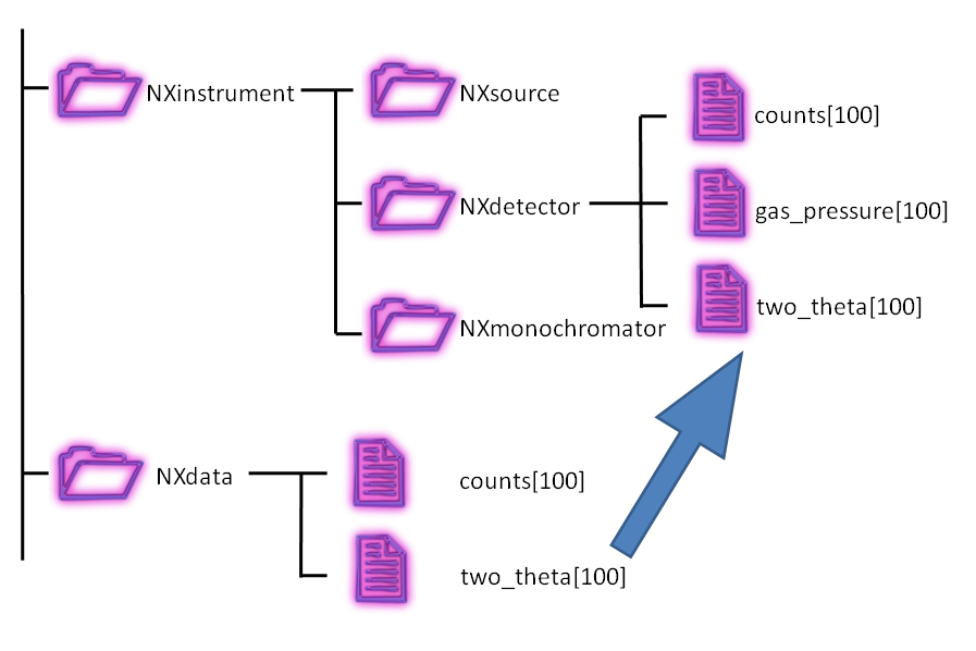
in the same file. For example: detector data is stored in the
NXinstrument/NXdetector group
but may be needed in NXdata for automatic plotting.
Rather then replicating the data, NeXus uses
links in such situations. See the figure for
a more descriptive representation of the concept of linking.
NeXus links are HDF5 hard links with an additional target attribute.
The target attribute is added [1] for NeXus to distinguish the HDF5 path to the
original[2] dataset. The value of the target attribute is the HDF5
path [3] to the original dataset.
NeXus links are best understood with an example.
The canonical location (expressed as a NeXus class path) to store wavelength
(see Strategies: The wavelength) has been:
/NXentry/NXinstrument/NXcrystal/wavelength
An alternative location for this field makes sense to many,
especially those not using a crystal to create monochromatic radiation:
/NXentry/NXinstrument/NXmonochromator/wavelength
These two fields might be hard linked together in a NeXus data file
(using HDF5 paths such /entry/instrument):
It is possible that the linked field or group has a
different name than the original. One obvious use of this capability
is to adapt to a specific requirement of an application definition.
For example, suppose some application definition required the
specification of wavelength as a field named lambda in the entry group.
This requirement can be satisifed easily:
NeXus also allows for links to external files.
Consider the case where an instrument uses a detector with
a closed-system software support provided by a commercial vendor.
This system writes its images into a NeXus HDF5 file.
The instrument’s data acquisition system writes instrument metadata
into another NeXus HDF5 file. In this case, the instrument metadata file
might link to the data in the detector image file.
Here is an example (from Diamond Light Source)
showing an external file link in HDF5:
Example of linking to data in an external HDF5 file
The NAPI code [5] makes no target attribute assignment for
links to external files. It is best to avoid using the
target attribute with external file links.
The NIAC is working at resolving the technical limitations
The NAPI maintains a group attribute @napimount that provides
a URL to a group in another file. More information about the
@napimount attribute is described in the
NeXus Programmers Reference. [6]
Consider the case described in
Links to Data in External HDF5 Files,
where numerical data are provided in two different HDF5 files and a master NeXus HDF5 file links to
the data through external file links. HDF5 will not allow hard links to be constructed with these data
objects in the master file. An error such as Interfile hard links are not allowed (as generated
from h5py) will arise. This makes sense since there is no such data object in the file.
Instead, it is necessary to make an external file link at each place in the master where external
data is to be represented.
Data groups often describe objects in the experiment (monitors, detectors,
monochromators, etc.), so that the contents (both fields and/or other
groups) comprise the properties of that object. NeXus has defined a set of standard
objects, or base classes,
out of which a NeXus file can be constructed. Each data group
is identified by a name and a class. The group class defines the type of object
and the properties that it can contain, whereas the group name defines a unique instance
of that class. These classes are
defined in XML using the NeXus Definition Language
(NXDL) format. All NeXus class types adopted by the NIAC must
begin with NX.
Classes not adopted by the NIAC must not
start with NX.
Note
NeXus base classes are the components used to build the
NeXus data structure.
Not all classes define physical objects. Some refer to logical groupings of
experimental information, such as
plottable data,
sample environment logs, beam profiles, etc.
There can be multiple instances of each class. On
the other hand, a typical NeXus file will only contain a small subset of the
possible classes.
Note
The groups, fields, links, and attributes of a base class
definition are all optional, with a few particular exceptions in
NXentry and NXdata. They are named in the specification
to describe the exact spelling and usage of the term when it appears.
NeXus base classes are not proper classes in the same sense as used in object oriented programming
languages. In fact the use of the term classes is actually misleading but has established itself during the
development of NeXus. NeXus base classes are rather dictionaries of field names and their meanings
which are permitted in a particular NeXus group implementing the NeXus class. This sounds complicated but
becomes easy if you consider that most NeXus groups describe instrument components. Then for example, a
NXmonochromator base class describes all the possible field names which NeXus allows to be used to describe a
monochromator.
Most NeXus base classes represent instrument components. Some are used as containers to structure information in a
file (NXentry, NXcollection, NXinstrument, NXprocess, NXparameters).
But there are some base classes which have special uses which need to be mentioned here:
NXlog is used to store time stamped data like the log of a temperature controller.
Basically you give a start time,
and arrays with a difference in seconds to the start time and the values read.
NXcollection is used to gather together any set of terms.
Anything (groups, fields, or attributes) placed in
an NXcollection group will not be validated.
One use is to use this as a container class for the various
control system variables from a beamline or instrument.
This group provides a place to store general notes, images, video or
whatever. A mime type is stored together with a binary blob of data.
Please use this only for auxiliary information, for example an image
of your sample, or a photo of your boss.
NXgeometry and its subgroups NXtranslation,
NXorientation, NXshape are used to store absolute positions in the
laboratory coordinate system or to define shapes.
These groups can appear anywhere in the NeXus hierarchy, where needed. Preferably close to the component they
annotate or in a NXcollection. All of the base classes are documented in the reference manual.
Single inheritance is supported in NeXus for both base classes and application definitions (which are
described below). Extending a base class or application definition inherits the properties and objects of the
parent class or definition, such as groups, fields, attributes, and symbol tables. These properties and objects
of the parent can then be overridden by the subclass. Only single inheritance is allowed (you can only inherit
from a single parent).
Use the @extends attribute of a definition to indicate which definition is being subclassed. Base classes
should extend from NXobject unless they are being subclassed.
The most notable special base class (or group in NeXus) is NXdata.
NXdata is the answer to a basic motivation of NeXus to facilitate
automatic plotting of data.
NXdata is designed to contain the main dataset and its associated
dimension scales (axes) of a NeXus data file.
The usage scenario is that an automatic data plotting program just
opens a NXentry and then continues to search for any NXdata
groups. These NXdata groups represent the plottable data.
An algorithm for identifying the default plottable data
is presented in the
chapter titled Rules for Storing Data Items in NeXus Files.
There are many ways to store metadata about your experiments.
Already there are many fields in the various base classes
to store the more common or general metadata, such as wavelength.
(For wavelength, see the Strategies: The wavelength section.)
One common scheme is to store the metadata all in one
group. If the group is to be validated for content,
then there are several possibilities, as shown in the next table:
The objects described so far provide us with the means to store data from a wide variety of instruments,
simulations, or processed data as resulting from data analysis. But NeXus strives to express strict standards for
certain applications of NeXus, too. The tool which NeXus uses for the expression of such strict standards is the NeXus
Application Definition.
A NeXus Application Definition describes which groups and data items have to be present in
a file in order to properly describe an application of NeXus. For example for describing a powder diffraction
experiment.
An application definition may also declare terms which are optional in the data file.
Typically an application definition will contain only a small subset of the many groups and fields
defined in NeXus. NeXus application definitions are also expressed in the NeXus Definition Language (NXDL). A tool exists
which allows one to validate a NeXus file against a given application definition.
Note
NeXus application definitions define the minimum required information
necessary to satisfy data analysis or other data processing.
Another way to look at a NeXus application definition is as a
contract between a file producer (writer) and a file consumer (reader).
The contract reads:
If you write your files following a particular NeXus application definition,
I can process these files with my software.
Yet another way to look at a NeXus application definition is to understand it as an interface definition
between data files and the software which uses this file. Much like an interface in the Java or other modern
object oriented programming languages.
Like base classes, NeXus supports Inheritance in NeXus in application definitions.
Please note that a NeXus Application Definition will only define the bare minimum of data necessary to perform
common analysis with data. Practical files will nearly always contain more data. One of the beauties of NeXus is
that it is always possible to add more data to a file without breaking its compliance with its application definition.
The NeXus coordinate system is shown below. Note that
it is the same as that used by McStas (http://mcstas.org). This choice is
arbitrary and any other choice should be possible as long as it is
used consistently and application code that reads NeXus files does not assume
any prior knowledge of the chosen coordinate system.
In the recommended way of dealing with geometry NeXus uses a series of
transformations to place objects in space.
In this world view, the absolute position of a component or a detector pixel with respect to
the laboratory coordinate system is calculated by applying a series of translations and
rotations. Thus a rotation or translation operation transforms the whole coordinate system
and gives rise to a new local coordinate system. These transformations between coordinate
systems are mathematical operations and can be expressed as matrices and their combination
as matrix multiplication. A very important aspect is that the order of application of the
individual operations does matter. The mathematics behind this is well known and used in
such applications such as industrial robot control, flight dynamics and
computer games. The beauty in this comes from the fact that the operations to apply map easily
to instrument settings and constants. It is also easy to analyze the contribution of each individual
operation: this can be studied under the condition that all other operations are at a zero setting.
In order to use coordinate transformations, several pieces of information need to be known:
Type
The type of operation: rotation or translation
Direction
The direction of the translation or the direction of the rotation axis
Value
The angle of rotation or the length of the translation
Order
The order of operations to apply to move a component into its place.
NeXus chooses to encode information about each transformation as a field in an NXtransformations
group in the following way:
value
This is represented in the actual data of the field or the value of the
transformation. Its actual name should relate to the physical device used to
effect the transformation.
The coordinate transformation attributes are:
transformation_type
This specifies the type of transformation and is either rotation
or translation and describes the kind of operation performed
vector (NX_NUMBER)
This is a set of 3 values forming a unit vector for direction that
describes the components of either the direction of the rotation axis or
the direction along which the translation happens.
offset (NX_NUMBER)
This is a set of 3 values forming the offset vector for a translation to apply
before applying the operation of the actual transformation. Without this offset
attribute, additional virtual translations would need to be introduced in order
to encode mechanical offsets in the axis.
depends_on
The order is encoded through this attribute. The value is the name of the
transformation upon which the current transformation depends on.
As each transformation represents possible motion by a physical device, this
dependency expresses the attachment order; thus, the current device is attached
to (or mounted on) the next device referred to by the attribute.
Allowed values for depends_on are:
.
A dot ends the depends_on chain
name
The name of a field within the enclosing group
dir/name
The name of a field further along the path
/dir/dir/name
An absolute path to a field in another group
In addition, for each beamline component, there is a depends_on attribute
that points to the field at the head of the axis dependency chain. For example,
consider an eulerian cradle as used on a four-circle diffractometer.
Such a cradle has a dependency chain of phi:chi:rotation_angle. Then
the depends_on field in NXsample would have the value phi.
NeXus Transformation encoding
Transformation encoding for an eulerian cradle on a four-circle diffractometer
The type and direction of the NeXus standard operations is documented below
in the table: Actions of standard NeXus fields.
The rule is to always give the attributes to make perfectly clear how the axes work. The CIF scheme
also allows to store and use arbitrarily named axes in a NeXus file.
The CIF scheme (see NXtransformations) is the preferred method
for expressing geometry in NeXus.
The shape of instrument components can be described using the NXoff_geometry
class. NXoff_geometry is a polygon-based description, based on the open OFF format.
Conversion between OFF files and the NeXus description is straightforward. This is
beneficial as existing tools can use, view or manipulate the geometry in OFF files.
CAD software, for example FreeCAD, can be used to
define the geometry. 3D rendering tools such as Geomview
can be used to view the geometry. McStas can use OFF
files to define the shape of components for scattering simulations.
The example OFF file shown below defines a cube. The first line containing
numbers defines: the number of vertices, the number of faces (polygons) making
up the model’s surface, and the number of edges in the mesh. Note, the number of
edges must be present but does not need to be correct
(http://www.geomview.org/docs/html/OFF.html).
Following the initial line are the xyz coordinates of each vertex, followed
by the list of faces. Each line defining a face starts with the number of
vertices in that face followed by the sequence number of the composing vertices,
indexed from zero. The vertex indices form a winding order by defining the face
normal by the right-hand rule. The number of vertices in each face need not be
constant; a mesh can comprise of polygons of many different orders.
The list of vertices in an OFF file maps directly to the vertices dataset in
the NXoff_geometry class. The vertex indices of the face list in the OFF
file occupy the winding_order dataset of the NeXus class, however the list
is flattened to 1D in order to avoid a ragged-edged dataset, which are not
easy to work with using HDF libraries. A faces dataset contains the position
of the first entry in winding_order for each face. The NXoff_geometry
equivalent of the OFF cube example is shown below.
Although the polygon-based description of NXoff_geometry is very flexible,
it is not ideal for curved shapes when high precision is required since a very
large number of vertices may be necessary. A common example of this is when
describing helium tube, neutron detectors. NXcylindrical_geometry provides
a more concise method of defining shape for such cases.
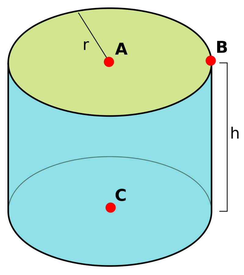
Like NXoff_geometry, NXcylindrical_geometry contains a vertices
dataset. The indices of three vertices (A, B, C in Cylinder definition with three vertices) in the vertices dataset are used to
define each cylinder in the cylinders dataset.
An NXoff_geometry or NXcylindrical_geometry group named detector_shape
can be placed in an NXdetector or NXdetector_module to define the complete
shape of the detector. Alternatively, the group can be named pixel_shape
and define the shape of a single pixel. In this case, x_pixel_offset,
y_pixel_offset and z_pixel_offset datasets of the NXdetector define
how the pixel shape is tiled to form the geometry of the complete detector.
The above system of chained transformations is the recommended way of
encoding geometry going forward. This section describes the traditional way
this was handled in NeXus, which you may find occasionally in old files.
Coordinate systems
in NeXus have undergone significant development. Initially, only motor
positions of the relevant motors were stored without further standardization.
This soon proved to be
too little and the NeXus polar coordinate system
was
developed. This system still
is very close to angles that are meaningful to an instrument scientist
but allows to define general positions of
components easily. Then users from the simulation community
approached the NeXus team and asked for a means
to store absolute coordinates. This was implemented through
the use of the NXgeometry class on top of the
McStas system.
We soon learned that all the things we do can be expressed through the
McStas coordinate system. So it became the reference coordinate system
for NeXus. NXgeometry was expanded to allow the description of shapes
when the demand came up. Later, members of the
CIF team
convinced the NeXus team of the beauty of transformation matrices and
NeXus was enhanced to store the necessary information to fully map CIF
concepts. Not much had to be changed though as we
choose to document the existing angles in CIF terms. The CIF system
allows to store arbitrary operations and nevertheless calculate
absolute coordinates in the laboratory coordinate system. It also
allows to convert from local, for example detector
coordinate systems, to absolute coordinates in the laboratory system.
As stated above, NeXus uses the
McStas coordinate system (http://mcstas.org)
as its laboratory coordinate system.
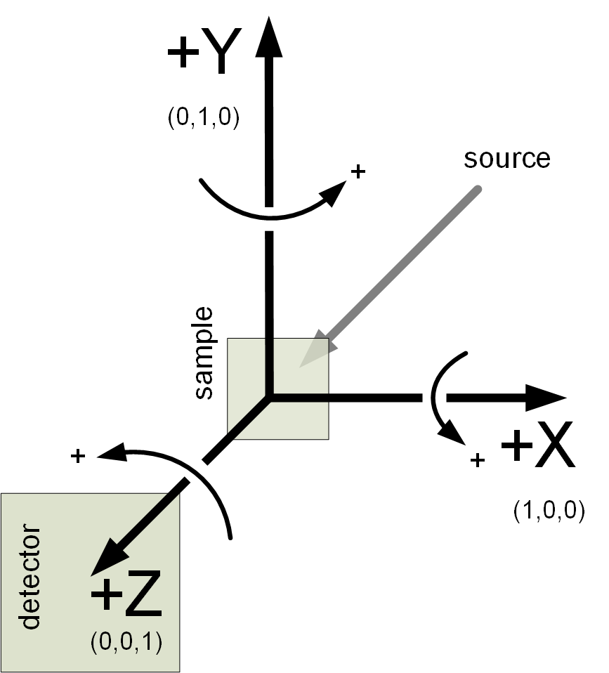
The instrument is given a global, absolute coordinate system where the
z axis points in the direction of the incident beam,
the x axis is perpendicular to the beam in the horizontal
plane pointing left as seen from the source, and the y axis
points upwards. See below for a drawing of the McStas coordinate system. The origin of this
coordinate system is the sample position or, if this is ambiguous, the center of the sample holder
with all angles and translations set to zero. The McStas coordinate system is
illustrated in the next figure:
The NeXus NXgeometry class directly uses the
McStas coordinate system.
NXgeometry classes can appear in any
component in order to specify its position.
The suggested name to use is geometry.
In NXgeometry the NXtranslation/values
field defines the absolute position of the component in the McStas coordinate system. The NXorientation/value field describes
the orientation of the component as a vector of in the McStas coordinate system.
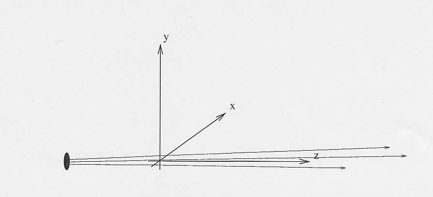
In this system,
the instrument is considered as a set of components through
which the incident beam passes. The variable distance is assigned to each component and represents the
effective beam flight path length between this component and the sample. A sign
convention is used where negative numbers represent components pre-sample and positive
numbers components post-sample. At each component there is local spherical coordinate system
with the angles polar_angle and azimuthal_angle.
The size of the sphere is the distance to the previous component.
In order to understand this spherical polar coordinate system it is helpful
to look initially at the common condition that azimuthal_angle
is zero. This corresponds to working directly in the horizontal scattering
plane of the instrument. In this case polar_angle maps
directly to the setting commonly known as two theta.
Now, there are instruments where components live outside of the scattering plane.
Most notably detectors. In order to describe such components we first apply
the tilt out of the horizontal scattering plane as the
azimuthal_angle. Then, in this tilted plane, we rotate
to the component. The beauty of this is that polar_angle
is always two theta. Which, in the case of a component
out of the horizontal scattering plane, is not identical to the value read
from the motor responsible for rotating the component. This situation is shown in
Polar Coordinate System.