1.2.3.2. Rules for Storing Data Items in NeXus Files
This section describes the rules which apply for storing single data items.
Naming Conventions
Group and field names used within NeXus follow a naming convention described by the following rules:
The names of NeXus group and field items must only contain a restricted set of characters.
This set is described by a regular expression syntax regular expression regular expression syntax, as described below.
For the class names [1] of NeXus group items, the prefix NX is reserved as shown in the table below. Thus all NeXus class names start with NX. The chapter titled NeXus: Reference Documentation lists the available NeXus class names as either base classes, application definitions, or contributed definitions.
NXDL group and field names
The names of NeXus group and field items are validated according to these boundaries:
Recommended names [3]
lower case words separated by underscores and, if needed, with a trailing number
NOTE: this is used by the NeXus base classes
Allowed names
any combination of upper and lower case letter, numbers, underscores and periods, except that periods cannot be at the start or end of the string
NOTE: this matches the validItemName regular expression below
Invalid names
NOTE: does not match the validItemName regular expression below
Regular expression pattern for NXDL group and field names
The NIAC recognises that the majority of the world uses characters outside of the basic latin (a.k.a. US-ASCII, 7-bit ASCII) set currently included in the allowed names. The restriction given here reflects current technical issues and we expect to revisit the issue and relax such restrictions in future.
The names of NeXus group and field items must match this regular expression (named validItemName in the XML Schema file: nxdl.xsd):
1^[a-zA-Z0-9_]([a-zA-Z0-9_.]*[a-zA-Z0-9_])?$
The length should be limited to no more than 63 characters (imposed by the HDF5 rules for names).
It is recognized that some facilities will construct data files with group and field names with upper case letters or start names with a number or include a period in a name. [3]
Use of underscore in descriptive names
Sometimes it is necessary to combine words in order to build a descriptive name for a field or a group. In such cases lowercase words are connected by underscores.
1number_of_lenses
For all fields, only names from the NeXus base class dictionaries should be used. If a field name or even a complete component is missing, please suggest the addition to the NIAC: The NeXus International Advisory Committee. The addition will usually be accepted provided it is not a duplication of an existing field and adequately documented.
Note
The NeXus base classes provide a comprehensive dictionary of terms that can be used for each class. The expected spelling and definition of each term is specified in the base classes. It is not required to provide all the terms specified in a base class. Terms with other names are permitted but might not be recognized by standard software. Rather than persist in using names not specified in the standard, please suggest additions to the NIAC: The NeXus International Advisory Committee.
The data stored in NeXus fields must be readback values.
This means values as read from the detector, other hardware, etc.
There are occasions where it is sensible to store the target value
the variable was supposed to have. In such cases, the
target value is stored with a name built by appending
_set to the NeXus (readback) field name.
Consider this example:
1temperature
2temperature_set
The temperature field will hold the readback from the
cryostat/furnace/whatever. The field temperature_set will hold
the target value for the temperature as set by the
experiment control software.
Some fields share a common part of their name and an additional part
name that makes the whole name specific. For example, a unit_cell
might have parts named abc, alphabetagamma, and volume. It
is recommended to write them with the common part first, an underscore
(_), and then the specific part. In this way, the fields will sort
alphabetically on the common name. So, in this example:
1unit_cell_abc
2unit_cell_alphabetagamma
3unit_cell_volume
Reserved prefixes
When naming an attribute, field, or group, NeXus has reserved certain prefixes to the names to ensure that names written in NeXus files will not conflict with future releases as the NeXus standard evolves. Prefixes should follow a naming scheme of uppercase letters followed by an underscore, but exceptions will be made for cases already in wide use. The following table lists the prefixes reserved by NeXus.
prefix |
use |
meaning |
URL |
|---|---|---|---|
|
attributes |
reserved for use by Bluesky project |
|
|
attributes, fields |
reserved for use by Dectris |
|
|
attributes |
reserved for use by pulsedTD Muon definition |
https://www.isis.stfc.ac.uk/Pages/nexus-definition-v27924.pdf |
|
attributes |
reserved for use by EPICS area detector |
|
|
NXDL class |
for the class names used with NeXus groups |
|
|
attributes |
reserved for use by NeXus |
|
|
attributes |
reserved for the US protein data bank |
|
|
attributes |
reserved for use by canSAS |
|
|
attributes |
reserved for use by silx |
Reserved suffixes
When naming a field, NeXus has reserved certain suffixes to the names
so that a specific meaning may be attached. Consider a field named DATASET,
the following table lists the suffixes reserved by NeXus.
suffix |
reference |
meaning |
|---|---|---|
|
end points of the motions that start with |
|
|
uncertainties (a.k.a., errors) |
|
|
intended average range through which the corresponding axis moves during the exposure of a frame |
|
|
Integer array that defines the indices of the signal field which need to be used in the |
|
|
Field containing a signal mask, where 0 means the pixel is not masked. If required, bit masks are defined in NXdetector |
|
|
Target value of |
|
|
divide |
Variants
Sometimes it is necessary to store alternate values of a NeXus field in a NeXus file. A common example may be the beam center of which a rough value is available at data acquisition. But later on, a better beam center is calculated as part of the data reduction. In order to store this without losing the historical information, the original field can be given a variant attribute that points to a new field containing the obsolete value. If even better values become available, further fields can be inserted into the chain of variant attributes pointing to the preceeding value for the field. A reader can thus keep the best value in the pre-defined field, and also be able to follow the variant chain and locate older variants.
A little example is in order to illustrate the scheme:
1beam_center_x
2        @variant=beam_center_x_refined
3beam_center_x_refined
4        @variant=beam_center_x_initial_guess
5beam_center_x_initial_guess
NeXus borrowed this scheme from CIF. In this way all the different variants of a field can be preserved. The expectation is that variants will be rarely used and NXprocess groups with the results of data reduction will be written instead.
Uncertainties or Errors
It is desirable to store experimental errors (also known as
uncertainties) together with the data. NeXus supports this through
a convention: uncertainties or experimental errors on data are
stored in a separate field which has a name consisting of the
original name of the data with _errors appended to it.
These uncertainties fields have the same shape as the original data field.
An example, from NXdetector:
1data
2data_errors
3beam_center_x
4beam_center_x_errors
Where data errors would contain the errors on data, and beam_center_x_errors the error on the beam center for x.
NeXus Array Storage Order
NeXus stores multi-dimensional arrays of physical values in C language storage order, where the first dimension has the slowest varying index when iterating through the array in storage order, and the last dimension is the fastest varying. This is the rule. Good reasons are required to deviate from this rule.
Where the array contains data from a detector, the array dimensions may correspond to physical directions or axes. The slowest, slow, fast, fastest qualifiers can then apply to these axes too.
It is possible to store data in storage orders other than C language order.
As well it is possible to specify that the data needs to be converted first before being useful. Consider one situation, when data must be streamed to disk as fast as possible and conversion to C language storage order causes unnecessary latency. This case presents a good reason to make an exception to the standard rule.
Non C Storage Order
In order to indicate that the storage order is different from C storage order two additional data set attributes, offset and stride, have to be stored which together define the storage layout of the data. Offset and stride contain rank numbers according to the rank of the multidimensional data set. Offset describes the step to make when the dimension is multiplied by 1. Stride defines the step to make when incrementing the dimension. This is best explained by some examples.
Offset and Stride for 1 D data:
 1   * raw data = 0 1 2 3 4 5 6 7 8 9
 2      size[1] = { 10 }  // assume uniform overall array dimensions
 3
 4   * default stride:
 5      stride[1] = { 1 }
 6      offset[1] = { 0 }
 7      for i:
 8         result[i]:
 9            0 1 2 3 4 5 6 7 8 9
10
11   * reverse stride:
12      stride[1] = { -1 }
13      offset[1] = { 9 }
14      for i:
15         result[i]:
16            9 8 7 6 5 4 3 2 1 0
Offset and Stride for 2D Data
 1   * raw data = 0 1 2 3 4 5 6 7 8 9 10 11 12 13 14 15 16 17 18 19
 2      size[2] = { 4, 5 }  // assume uniform overall array dimensions
 3
 4   * row major (C) stride:
 5      stride[2] = { 5, 1 }
 6      offset[2] = { 0, 0 }
 7      for i:
 8         for j:
 9            result[i][j]:
10               0 1 2 3 4
11               5 6 7 8 9
12               10 11 12 13 14
13               15 16 17 18 19
14
15   * column major (Fortran) stride:
16      stride[2] = { 1, 4 }
17      offset[2] = { 0, 0 }
18      for i:
19         for j:
20            result[i][j]:
21               0 4 8 12 16
22               1 5 9 13 17
23               2 6 10 14 18
24               3 7 11 15 19
25
26   * "crazy reverse" row major (C) stride:
27      stride[2] = { -5, -1 }
28      offset[2] = { 4, 5 }
29      for i:
30         for j:
31            result[i][j]:
32               19 18 17 16 15
33               14 13 12 11 10
34               9 8 7 6 5
35               4 3 2 1 0
Offset and Stride for 3D Data
 1  * raw data = 0 1 2 3 4 5 6 7 8 9 10 11 12 13 14 15 16 17 18 19
 2         20 21 22 23 24 25 26 27 28 29 30 31 32 33 34 35 36 37 38 39
 3         40 41 42 43 44 45 46 47 48 49 50 51 52 53 54 55 56 57 58 59
 4      size[3] = { 3, 4, 5 }  // assume uniform overall array dimensions
 5
 6   * row major (C) stride:
 7      stride[3] = { 20, 5, 1 }
 8      offset[3] = { 0, 0, 0 }
 9      for i:
10         for j:
11            for k:
12               result[i][j][k]:
13                  0 1 2 3 4
14                  5 6 7 8 9
15                  10 11 12 13 14
16                  15 16 17 18 19
17
18                  20 21 22 23 24
19                  25 26 27 28 29
20                  30 31 32 33 34
21                  35 36 37 38 39
22
23                  40 41 42 43 44
24                  45 46 47 48 49
25                  50 51 52 53 54
26                  55 56 57 58 59
27
28   * column major (Fortran) stride:
29      stride[3] = { 1, 3, 12 }
30      offset[3] = { 0, 0, 0 }
31      for i:
32         for j:
33            for k:
34               result[i][j][k]:
35                  0 12 24 36 48
36                  3 15 27 39 51
37                  6 18 30 42 54
38                  9 21 33 45 57
39
40                  1 13 25 37 49
41                  4 16 28 40 52
42                  7 19 31 43 55
43                  10 22 34 46 58
44
45                  2 14 26 38 50
46                  5 17 29 41 53
47                  8 20 32 44 56
48                  11 23 35 47 59
NeXus Data Types
description |
matching regular expression |
|---|---|
integer |
|
floating-point |
|
array |
|
valid item name |
|
valid class name |
|
NeXus supports numeric data as either integer or floating-point numbers. A number follows that indicates the number of bits in the word. The table above shows the regular expressions that match the data type specifier.
- integers
NX_INT8,NX_INT16,NX_INT32, orNX_INT64
- floating-point numbers
NX_FLOAT32orNX_FLOAT64
- date / time stamps
NX_DATE_TIMEorISO8601: Dates and times are specified using ISO-8601 standard definitions. Refer to NeXus dates and times.
- strings
NX_CHAR: The preferred string representation is UTF-8. Both fixed-length strings and variable-length strings are valid. String arrays cannot be used where only a string is expected (title, start_time, end_time,NX_classattribute,…). Fields or attributes requiring the use of string arrays will be clearly marked as such (like theNXdataattribute auxiliary_signals).
- binary data
Binary data is to be written as
UINT8.
- images
Binary image data is to be written using
UINT8, the same as binary data, but with an accompanying image mime-type. If the data is text, the line terminator is[CR][LF].
NeXus dates and times
NeXus dates and times
should be stored using the ISO 8601 [5] format,
e.g. 1996-07-31T21:15:22+0600 (which includes
a time zone offset of +0600).
Note: The time zone offset is always numeric or Z (which means UTC).
The standard also allows for time intervals in fractional seconds
with 1 or more digits of precision.
This avoids confusion, e.g. between U.S. and European conventions,
and is appropriate for machine sorting.
It is recommended to add an explicit time zone,
otherwise the local time zone is assumed per ISO8601.
The norm is that if there is no time zone, it is assumed
local time, however, when a file moves from one country to
another it is undefined. If the local time zone is written,
the ambiguity is gone.
strftime() format specifiers for ISO-8601 time
%Y-%m-%dT%H:%M:%S%z
Note
Note that the T appears literally in the string,
to indicate the beginning of the time element, as specified
in ISO 8601. It is common to use a space in place of the
T, such as 1996-07-31 21:15:22+0600.
While human-readable (and later allowed in a relaxed revision
of the standard), compatibility with libraries supporting
the ISO 8601 standard is not
assured with this substitution. The strftime()
format specifier for this is “%Y-%m-%d %H:%M:%S%z”.
NeXus Data Units
Given the plethora of possible applications of NeXus, it is difficult to
define units to use. Therefore, the general rule is that you are free to
store data in any unit you find fit. However, any field must have a
units attribute which describes the units. Wherever possible, SI units are
preferred. NeXus units are written as a string attribute (NX_CHAR)
and describe the engineering units. The string
should be appropriate for the value.
Values for the NeXus units must be specified in
a format compatible with Unidata UDunits [6]
Application definitions may specify units to be used for fields
using an enumeration.
Storing Detectors
There are very different types of detectors out there. Storing their data
can be a challenge. As a general guide line: if the detector has some
well defined form, this should be reflected in the data file. A linear
detector becomes a linear array, a rectangular detector becomes an
array of size xsize times ysize.
Some detectors are so irregular that this
does not work. Then the detector data is stored as a linear array, with the
index being detector number till ndet. Such detectors must be accompanied
by further arrays of length ndet which give
azimuthal_angle, polar_angle and distance for each detector.
If data from a time of flight (TOF) instrument must be described, then the
TOF dimension becomes the last dimension, for example an area detector of
xsize vs. ysize
is stored with TOF as an array with dimensions
xsize, ysize,
ntof
.
Monitors are Special
Monitors, detectors that measure the properties
of the experimental probe rather than the probe’s interaction with the
sample, have a special place in NeXus files. Monitors are crucial to normalize data.
To emphasize their role, monitors are not stored in the
NXinstrument hierarchy but on NXentry level
in their own groups as there might be multiple monitors. Of special
importance is the monitor in a group called control.
This is the main monitor against which the data has to be normalized.
This group also contains the counting control information,
i.e. counting mode, times, etc.
Monitor data may be multidimensional. Good examples are scan monitors where a monitor value per scan point is expected or time-of-flight monitors.
Find the plottable data
Simple plotting is one of the motivations for the NeXus standard. To implement simple plotting, a mechanism must exist to identify the default data for visualization (plotting) in any NeXus data file. Over its history the NIAC has agreed upon a method of applying metadata to identify the default plottable data. This metadata has always been specified as HDF attributes. With the evolution of the underlying file formats and the NeXus data standard, the method to identify the default plottable data has evolved, undergoing three distinct versions.
- version 1:
Associating plottable data by dimension number using the axis attribute
- version 2:
- version 3:
Associating plottable data using attributes applied to the NXdata group
Consult the NeXus API section, which describes the routines available to program these operations. In the course of time, generic NeXus browsers will provide this functionality automatically.
For programmers who may encounter NeXus data files written using any of these methods, we present the algorithm for each method to find the default plottable data. It is recommended to start with the most recent method, Version 3, first.
Version 3
The third (current) method to identify the default plottable data is as follows:
Start at the top level of the NeXus data file (the root of the HDF5 hierarchy).
Pick the default NXentry group.
If the root has an attribute
default, the attribute’s value is the name of theNXentrygroup to be used. (The value of thedefaultattribute names an existing child of this group. The child group must itself be a NeXus group.) If no default attribute exists, pick anyNXentrygroup. This is trivial if there is only oneNXentrygroup.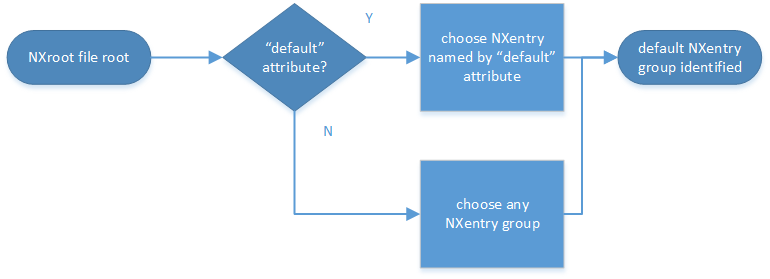
Find plottable data: select the
NXentrygroup¶Pick the default NXdata group.
Open the
NXentrygroup selected above. If it has an attributedefault, the attribute’s value is the name of theNXdatagroup to be used. (The value of thedefaultattribute names an existing child of this group. The child group must itself be a NeXus group.) If no default attribute exists, pick anyNXdatagroup. This is trivial if there is only oneNXdatagroup.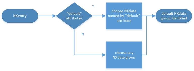
Find plottable data: select the
NXdatagroup
Pick the default plottable field (the signal data).
Open the
NXdatagroup selected above. If it has asignalattribute, the attribute’s value is the name of the field to be plotted. (The value of thesignalattribute names an existing child of this group. The child group must itself be a NeXus field.) If nosignalattribute is present on theNXdatagroup, then proceed to try an older NeXus method to find the default plottable data.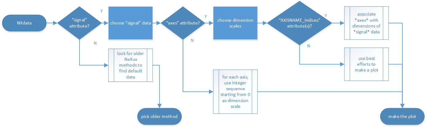
Find plottable data: select the signal data
Pick the fields with the dimension scales (the axes).
If the same
NXdatagroup has an attributeaxes, then its value is a string (signal data is 1-D) or string array (signal data is 2-D or higher rank) naming the field in this group to be used as dimension scales of the default plottable data. The number of values given must be equal to the rank of the signal data. These are the abscissae of the plottable signal data.If no field is available to provide a dimension scale for a given dimension, then a “
.” will be used in that position. In such cases, programmers are expected to use an integer sequence starting from 0 for each position along that dimension.Associate the dimension scales with each dimension of the plottable data.
For each field (its name is AXISNAME) in
axesthat provides a dimension scale, there will be anNXdatagroup attributeAXISNAME_indiceswhich value is an .. integer or integer array with value of the dimensions of the signal data to which this dimension scale applies.If no
AXISNAME_indicesattribute is provided, a programmer is encouraged to make best efforts assuming the intent of thisNXdatagroup to provide a default plot. TheAXISNAME_indicesattribute is only required when necessary to resolve ambiguity.It is possible there may be more than one
AXISNAME_indicesattribute with the same value or values. This indicates the possibilty of using alternate abscissae along this (these) dimension(s). The field named in theaxesattribute indicates the intention of the data file writer as to which field should be used by default.
Plot the signal data, given axes and AXISNAME_indices.
When all the default and signal attributes are present, this
Python code example will identify directly the default plottable data
(assuming a plot() function has been defined by some code:
group = h5py.File(hdf5_file_name, "r")

while "default" in group.attrs:
    child_group_name = group.attrs["default"]
    group = group[child_group_name]

# assumes group.attrs["NX_class"] == "NXdata"
signal_field_name = group.attrs["signal"]
data = group[signal_field_name]

plot(data)
Version 2
Tip
Try this method for older NeXus data files and Version 3 fails..
The second method to identify the default plottable data is as follows:
Start at the top level of the NeXus data file.
Loop through the groups with class
NXentryuntil the next step succeeds.
Find plottable data: pick a
NXentrygroup¶Open the NXentry group and loop through the subgroups with class
NXdatauntil the next step succeeds.
Find plottable data: pick a
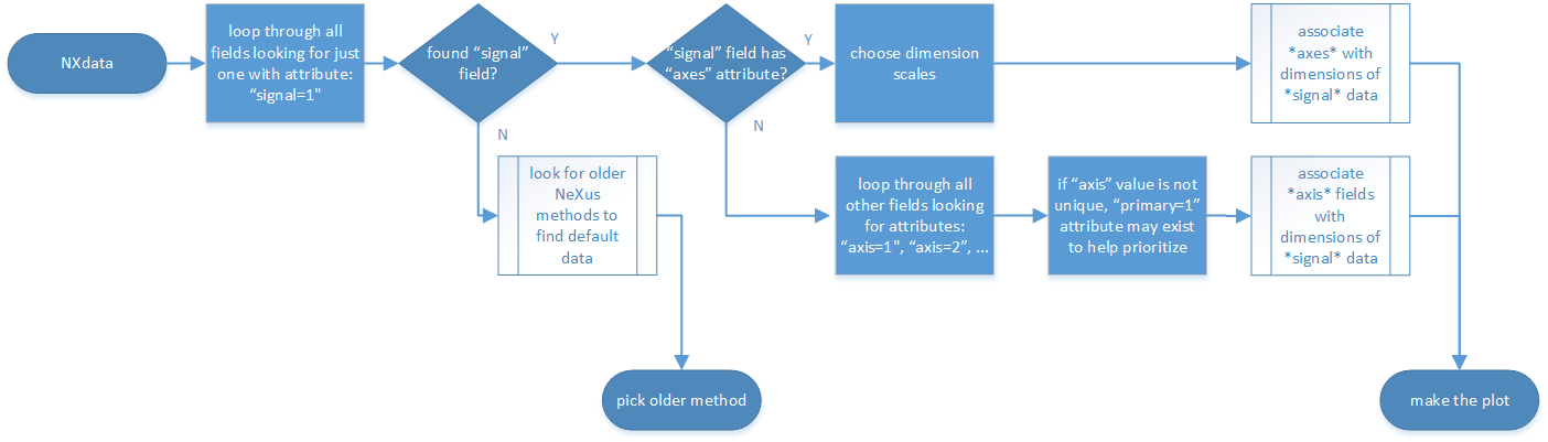
NXdatagroup¶Open the NXdata group and loop through the fields for the one field with attribute
signal="1". Note: There should be only one field that matches.This is the default plottable data.
If there is no such
signal="1"field, proceed to try an older NeXus method to find the default plottable data.If this field has an attribute
axes:The
axesattribute value contains a colon (or comma) delimited list (in the C-order of the data array) with the names of the dimension scales associated with the plottable data. Such as:axes="polar_angle:time_of_flight"Parse
axesand open the fields to describe your dimension scales
If this field has no attribute
axes:Search for fields with attributes
axis=1,axis=2, etc.These are the fields describing your axis. There may be several fields for any axis, i.e. there may be multiple fields with the attribute
axis=1. Among them the field with the attributeprimary=1is the preferred one. All others are alternative dimension scales.
Having found the default plottable data and its dimension scales: make the plot.
Find plottable data: select the signal data
Version 1
Tip
Try this method for older NeXus data files.
The first method to identify the default plottable data is as follows:
Open the first top level NeXus group with class
NXentry.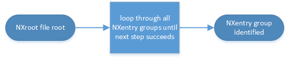
Find plottable data: pick the first
NXentrygroup¶Open the first NeXus group with class
NXdata.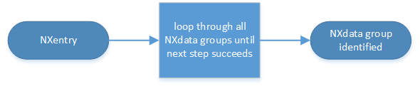
Find plottable data: pick the first
NXdatagroup¶Loop through NeXus fields in this group searching for the item with attribute
signal="1"indicating this field has the plottable data.Search for the one-dimensional NeXus fields with attribute
primary=1. These are the dimension scales to label the axes of each dimension of the data.Link each dimension scale to the respective data dimension by the
axisattribute (axis=1,axis=2, … up to the rank of the data).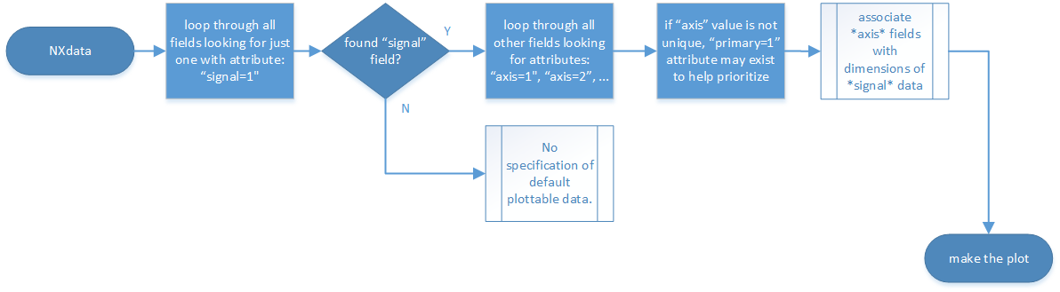
Find plottable data: select the signal data
If necessary, close this
NXdatagroup, search the nextNXdatagroup, repeating steps 3 to 5.If necessary, close the
NXentrygroup, search the nextNXentrygroup, repeating steps 2 to 6.
Associating Multi Dimensional Data with Axis Data
NeXus allows for storage of multi dimensional arrays of data. It is this data that presents the most challenge for description. In most cases it is not sufficient to just have the indices into the array as a label for the dimensions of the data. Usually the information which physical value corresponds to an index into a dimension of the multi dimensional data set. To this purpose a means is needed to locate appropriate data arrays which describe what each dimension of a multi dimensional data set actually corresponds too. There is a standard HDF facility to do this: it is called dimension scales. Unfortunately, when NeXus was first designed, there was only one global namespace for dimension scales. Thus NeXus had to devise its own scheme for locating axis data which is described here. A side effect of the NeXus scheme is that it is possible to have multiple mappings of a given dimension to physical data. For example, a TOF data set can have the TOF dimension as raw TOF or as energy.
There are now three methods of associating each data dimension to its respective dimension scale. Only the first method is recommended now, the other two (older methods) are now discouraged.
Associating plottable data using attributes applied to the NXdata group
Associating plottable data by dimension number using the axis attribute
The recommended method uses the axes attribute applied to the NXdata group
to specify the names of each
dimension scale.
A prerequisite is that the fields describing the axes of the plottable data
are stored together with the plottable data in the same NeXus group.
If this leads to data duplication, use links.
Associating plottable data using attributes applied to the NXdata group
Tip
Recommended: This is the “NIAC2014” method recommended for all new NeXus data files.
The default data to be plotted (and any associated axes) is specified using attributes attached to the NXdata group.
signal:Defines the name of the default field in the NXdata group. A field of this name must exist (either as field or link to field).
It is recommended to use this attribute rather than adding a signal attribute to the field. [7] The procedure to identify the default data to be plotted is quite simple. Given any NeXus data file, any
NXentry, or anyNXdata, follow the chain as it is described from that point. Specifically:The root of the NeXus file may have a
defaultattribute that names the default NXentry group. This attribute may be omitted if there is only one NXentry group. If a second NXentry group is later added, thedefaultattribute must be added then.Every NXentry group may have a
defaultattribute that names the default NXdata group. This attribute may be omitted if there is only one NXdata group or if no NXdata is present. If a second NXdata group is later added, thedefaultattribute must be added then.Every NXdata group will have a
signalattribute that names the field name to be plotted by default. This attribute is required.
axes:String array [8] that defines the independent data fields used in the default plot for all of the dimensions of the signal field. One entry is provided for every dimension in the signal field.
The field(s) named as values (known as “axes”) of this attribute must exist. An axis slice is specified using a field named
AXISNAME_indicesas described below (where the text shown here asAXISNAMEis to be replaced by the actual field name).When no default axis is available for a particular dimension of the plottable data, use a “.” in that position.
See examples provided on the NeXus webpage ([9]).
If there are no axes at all (such as with a stack of images), the axes attribute can be omitted.
AXISNAME_indices:Each
AXISNAME_indicesattribute indicates the dependency relationship of theAXISNAMEfield (whereAXISNAMEis the name of a field that exists in thisNXdatagroup) with one or more dimensions of the plottable data.Integer array [8] that defines the indices of the signal field (that field will be a multidimensional array) which need to be used in the
AXISNAMEfield in order to reference the corresponding axis value.The first index of an array is
0(zero).Here, AXISNAME is to be replaced by the name of each field described in the
axesattribute. An example with 2-D data, \(d(t,P)\), will illustrate:data_2d:NXdata @signal="data" @axes=["time","pressure"] @time_indices=0 @pressure_indices=1 data: float[1000,20] time: float[1000] pressure: float[20]
This attribute is to be provided in all situations. However, if the indices attributes are missing (such as for data files written before this specification), file readers are encouraged to make their best efforts to plot the data. Thus the implementation of the
AXISNAME_indicesattribute is based on the model of “strict writer, liberal reader”.
Examples
Several examples are provided to illustrate this method. More examples are available in the NeXus webpage ([9]).
simple 1-D data example showing how to identify the default data (counts vs. mr)
In the first example, storage of a 1-D data set (counts vs. mr) is described.
 1datafile.hdf5:NeXus data file
 2  @default="entry"
 3  entry:NXentry
 4    @default="data"
 5    data:NXdata
 6      @signal="counts"
 7      @axes="mr"
 8      @mr_indices=0
 9      counts: float[100]  --> the default dependent data
10      mr: float[100]      --> the default independent data
2-D data example showing how to identify the default data and associated dimension scales
A 2-D data set, data as a function of time and pressure is described.
By default as indicated by the axes attribute,
pressure is to be used.
The temperature array is described as a substitute for pressure
(so it replaces dimension 1 of data as indicated by the
temperature_indices attribute).
 1datafile.hdf5:NeXus data file
 2  @default="entry"
 3  entry:NXentry
 4    @default="data_2d"
 5    data_2d:NXdata
 6      @signal="data"
 7      @axes=["time","pressure"]
 8      @pressure_indices=1
 9      @temperature_indices=1
10      @time_indices=0
11      data: float[1000,20]
12      pressure: float[20]
13      temperature: float[20]
14      time: float[1000]
Associating plottable data by name using the axes attribute
Warning
Discouraged: See this method: Associating plottable data using attributes applied to the NXdata group.
This method defines an attribute of the data field
called axes.
The axes attribute contains the names of
each dimension scale
as a colon (or comma) separated list in the order they appear in C.
For example:
denoting axes by name
1  data:NXdata
2    time_of_flight = 1500.0 1502.0 1504.0 ...
3    polar_angle = 15.0 15.6 16.2 ...
4    some_other_angle = 0.0 0.0 2.0 ...
5    data = 5 7 14 ...
6      @axes = ["polar_angle", "time_of_flight"]
7      @signal = 1
Associating plottable data by dimension number using the axis attribute
Warning
Discouraged: See this method: Associating plottable data by name using the axes attribute
The original method defines an attribute of each dimension
scale field called axis.
It is an integer whose value is the number of
the dimension, in order of
fastest varying dimension.
That is, if the array being stored is data with elements
data[j][i] in C and
data(i,j) in Fortran, where i is the
time-of-flight index and j is
the polar angle index, the NXdata group
would contain:
denoting axes by integer number
 1  data:NXdata
 2    time_of_flight = 1500.0 1502.0 1504.0 ...
 3      @axis = 1
 4      @primary = 1
 5    polar_angle = 15.0 15.6 16.2 ...
 6      @axis = 2
 7      @primary = 1
 8    some_other_angle = 0.0 0.0 2.0 ...
 9      @axis = 1
10    data = 5 7 14 ...
11      @signal = 1
The axis attribute must
be defined for each dimension scale.
The primary attribute is unique to this method.
There are limited circumstances in which more
than one dimension scale
for the same data dimension can be included in the same NXdata group.
The most common is when the dimension scales are
the three components of an
(hkl) scan. In order to
handle this case, we have defined another attribute
of type integer called
primary whose value determines the order
in which the scale is expected to be chosen for plotting, i.e.
1st choice:
primary=12nd choice:
primary=2etc.
If there is more than one scale with the same value of the axis attribute, one
of them must have set primary=1. Defining the primary
attribute for the other scales is optional.
Note
- The
primaryattribute can only beused with the first method of defining
- dimension scales
discussed above. In addition to the
signaldata, this group could contain a data set of the same rank and dimensions callederrorscontaining the standard deviations of the data.